Many of us (if not all), use Google Sheets as a database, and we use it to store data for our projects. But sometimes you need more than just simple data storage. You want to get the value from one cell or range, based on another cell or range. This is where the Lookup function comes into play.
In this tutorial, I will show you how to do that using Google Sheet’s built-in function LOOKUP.
Let’s start!
What does LOOKUP do?
In a few words, LOOKUP uses two ranges to search for a given key in one range and outputs the corresponding value (the one in the same row) in the second range.
This seems an easy task, but unfortunately, this function is not always intuitive, and you should be very careful when using it. Let’s see why and then some simple examples on how to use it properly.
Why you should be careful when using this function
Lookup is a “strange” function, it can be very powerful, but you need to understand carefully how it works, or you’ll get strange/wrong data and not understand why or even not notice it. Even the Google help page is not too clear with the behavior of this function.
The first thing you need to know about lookup is that its result depends on the order in which your data is stored. This function assumes that you have an ordered list of values, so if it’s not, you can get strange results. This can be a big limitation, as if you have your data ordered by a column, and want to make a lookup from another column, you won’t be able to do it.
So, what happens when you use lookup?
When you use lookup, it returns the value from the first row that matches the criteria you specified. If there are no matching rows, it returns the nearest one that’s smaller than the search value. If there’s not a smaller value, you’ll get an Error and N/A value.
I know this is not easy to understand at first sight, but we’ll see some examples to understand it better!
How to use the LOOKUP function in Google Sheets
To better understand how this function works, we’ll use a simple spreadsheet with some sample data. You’ll probably have a bigger dataset, but this is enough to make some good examples.
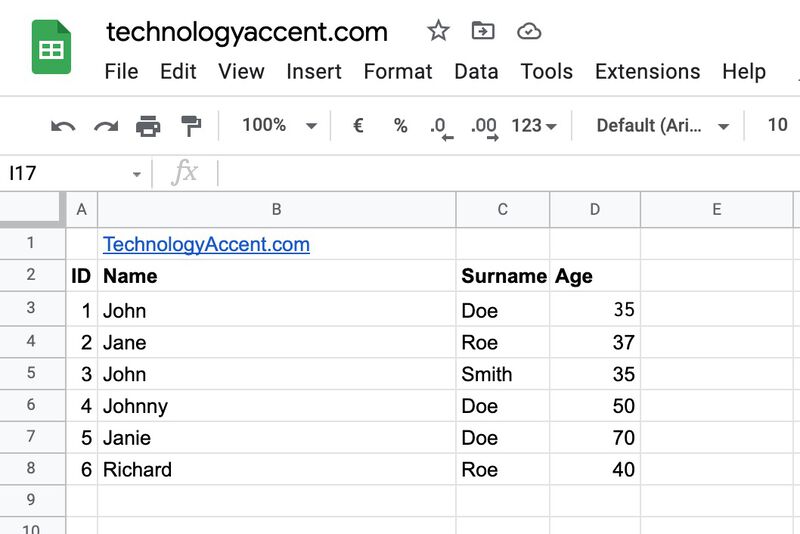
We have an ordered numerical ID column, two unordered textual columns for Name and Surname, and an unordered numerical age column.
The syntax
The syntax of the LOOKUP function is simple:
LOOKUP(search_key; search_range|search_result_array; [result_range])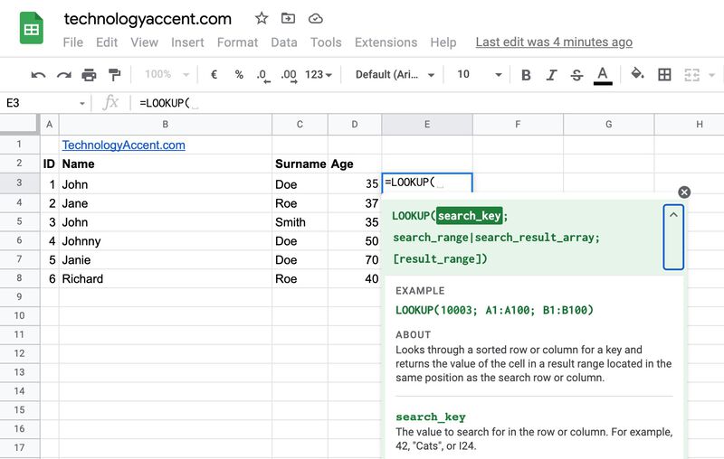
Let’s try to see what each argument means:
- search_key: this is the text we’re searching for, it can be “5”, “Johnny”, “38”, or any other value. Always remember the double quotes when you’re using a textual value.
- search_range or search_result_array: This is where things get a bit more complicated. You can use this argument to specify the search range. The function will search the search_key in the first column of the specified range.
- result_range: This parameter is optional, and it has to contain a single-column or single-row range. The function will pick as a result, the value in this range on the same row where the key has been found on the search_range. If you omit this parameter, the last column/row of the search_result_array will be used as a default.
This may sound complicated, but this is one of those things that are “better done than said”, so let’s pick some examples and everything will be clearer.
Basic syntax example
In the first example, we will try to get the name field given the person’s ID.
The syntax for this is simple and will help us to understand better how the function works.
=LOOKUP(2; A3:A8; B3:B8)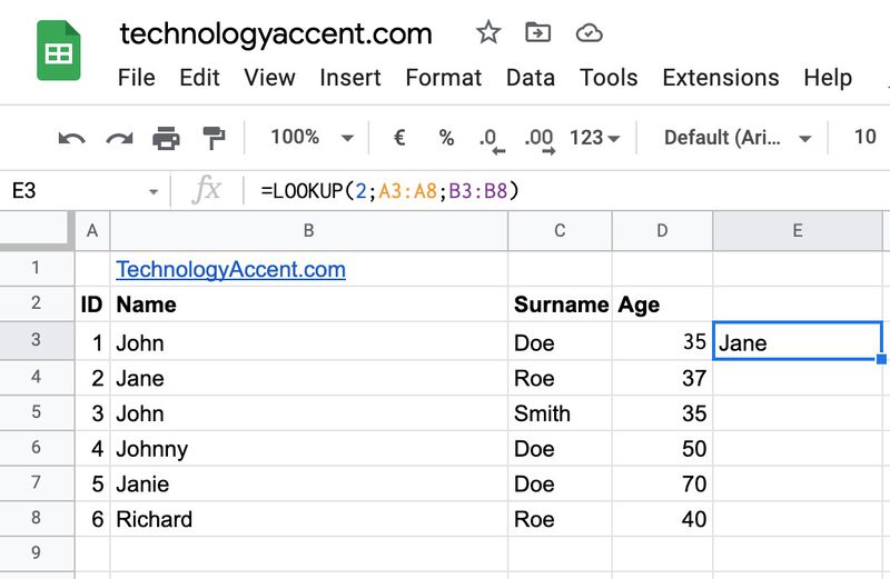
As you can see, we’re looking for the value 2 in the range A3:A8, and we want as a result the corresponding value from the range B3:B8.
Now let’s get to the shorter syntax, and try to get the same result with only the first two arguments:
Syntax without the result_range parameter
Without using the result_range parameter, we have to tell to LOOKUP both the A3:A8 and B3:B8 ranges in a single parameter.
=LOOKUP(2; A3:B8)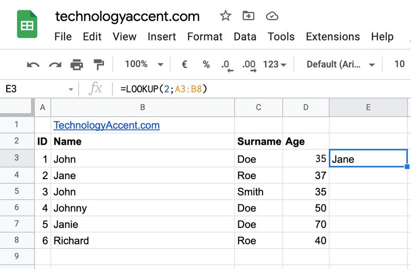
The result is the same, but with a shorter formula. Let’s analyze it
This time we used only the search_result_array parameter. The range takes the data in columns A and B. The behavior of the function, when it gets only one range, is to search on the first column (A in this case), and return the value from the last column (B in this case).
Understanding why ordered data is important
The LOOKUP function relies on the assumption that the search range is ordered from the smallest value to the largest. To better understand this, we can make some examples using the Age column on our demo spreadsheet.
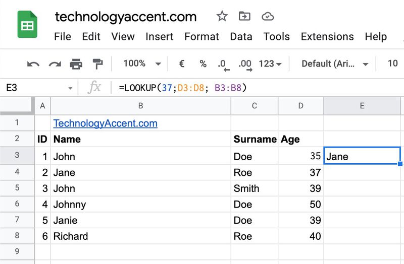
If we need to search for the name of the person with 37 years, we would probably write this function:
=LOOKUP(37;D3:D8; B3:B8)And get the right result
But if we try to find the person with 40 years (Richard), we’ll get into trouble…
=LOOKUP(40;D3:D8; B3:B8)Will give us…
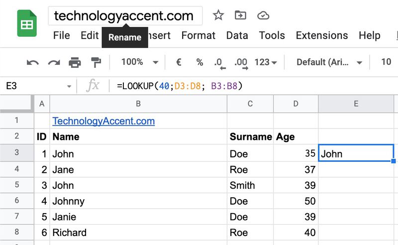
John!!! that’s completely wrong! What happened?
We can try to understand by following the function’s algorithm…
The algorithm starts to check the first cell (D3), and it doesn’t match with 40, then continues, until D6 is reached. At this point, the algorithm realizes that 50 is greater than 40, and using the assumption that the records are ordered, it assumes that from D6 to D8 all the numbers will be greater or equals to 50, so greater than 40. With this assumption, the algorithm goes one step back and takes the previous value that is lower than 40. The 39 of D5 is used, and the corresponding value is B5 containing John.
This is a strange behavior you need to always keep in mind when using this function on Google Sheets, as without an exact match the function silently fails and returns a value that could be wrong for us without any warning. In this example it’s evident because the dataset is small, but with a large range of cells, it can be a problem.
What if the first value in the column is larger than the search key?
We observed that if the exact match can’t be found, Google Sheets uses the nearest match taking the first value lower than the search key. But what happens if there’s no lower value? Let’s try with our example:
=LOOKUP(33;D3:D8; B3:B8)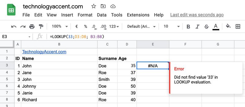
This time we finally got an error!
What happened this time is: The algorithm started with D3 as usual, and found that 35 is already greater than the searched 33. It then didn’t find a lower match, and couldn’t give us the nearest match, so we finally got an error “Did not find value 33 in LOOKUP evaluation”.
Using text as a search key
We started with numbers, as it’s probably easier to see why ordering is important and the various issues with LOOKUP. But the usage of LOOKUP is not restricted to searching for numbers, you can also use text as a search key. In this case, the ordering is still important and should be alphabetical.
The first example is a simple one: We want the surname of Richard.
=LOOKUP("Richard";B3:B8; C3:C8)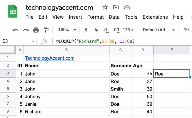
The result is the one we expect, as there’s no Name preceding Richard in alphabetical order on the list.
With text you need an exact match
If we order the data by name (as Google Sheets wants), but give a partial string, we get the wrong result:
=LOOKUP("Jani";B3:B8;C3:C8)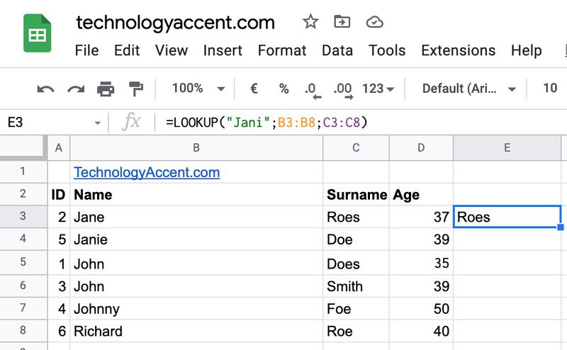
This happens because by default the LOOKUP formula expects an exact match. It’s a simple thing, but we’re all used to search engines and other tools guessing partial matches and sometimes we can forget when we need to enter the exact term.
This article is part of our productivity tips for Google Sheets series. You can find them all on our Tips and tricks for Google Sheets page.
Lookup rows instead of columns
The LOOKUP function works even for “horizontal data”. It’s not the most used way to represent data in a spreadsheet, but it works, you just need to select horizontal ranges instead of vertical ones.
Using VLOOKUP and HLOOKUP instead of LOOKUP.
There are two different functions in Google Sheets similar to the one we just analyzed: VLOOKUP (Vertical lookup) and HLOOKUP (Horizontal lookup).
The functions are similar, but there are some key differences that you probably would like to analyze. For many cases, one of these two functions can be a better choice for your spreadsheet.
Conclusions
The LOOKUP is a particular function, it makes Google Sheets powerful, but with its sometimes strange behaviors is also a dangerous one, prone to errors. Its silent mode of failing adds the risk of making a mistake and not noticing it, so always pay attention when you use it!