Google Sheets is a great tool for data analysis, but it can also be used to create beautiful charts and graphs. In this article, I’ll show you how to format numbers in Google Sheets using leading zeros.
Normally zeros in front of a number are meaningless. However, there are some use cases where you need them to be added, so you type 001, and Google Sheets keeps removing these mathematically meaningless zeros, replacing your 001 with just 1. How to solve this problem? Keep reading and we will discover it together!
Table of Contents
- Why should I add leading zeros in Google Sheets?
- Adding leading zeros without losing number format
- Adding leading zeros losing number format
Why should I add leading zeros in Google Sheets?
There’s no universal solution, as there are different use cases that could require you to add leading zeros to a number. We can separate these use cases into two main types. This separation will help you to identify the best solution for your needs.
Your number is a number you have to include in formulas
This is the case of simple numbers you want to be able to treat like mathematical numbers, including them in other formulas, operations, etc.
In this situation, the leading zeros are normally added just for visual purposes, normally to make all the numbers in a column the same length.
Your number is not a number, but just a “numeric text”
This is the case if you’re working with something like an id, a zip code, a bank account number, a credit card number, and similar numbers. Being these codes and not numbers, often the leading zeros are part of the code, so you have to keep them to preserve the code’s meaning.
The main point of these is that they are not “mathematic” numbers, you don’t need to make mathematical operations with them. So in your spreadsheet, you can handle these numbers like simple text strings.
These two different situations can be handled in different ways, so we will separate the proposed solutions into the ones preserving the “number” essence and the ones treating the number as text. You will probably be able to use the “number” solutions in “text” cases, but probably not the other way around.
Adding leading zeros without losing number format
Ok, you have some numbers you want to format in a pretty way making them all the same length, but you want to preserve the ability to apply formulas to them. Let’s see how to do it.
Using number format to add leading zeros
The easiest way to add leading zeros preserving the number format is for sure the custom number format method.
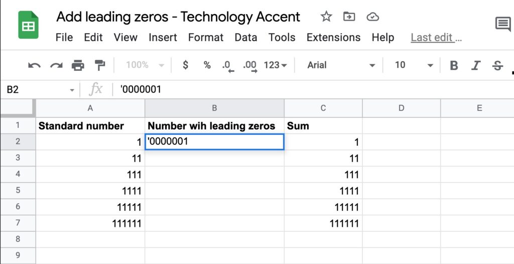
Let’s see our test spreadsheet:
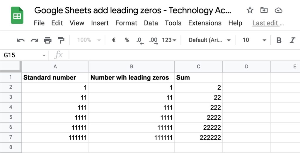
We have a column where we will preserve the standard number format, one where we will work to add leading zeros with the different methods, and one with the sum of the preceding cells, so we can test if the column with leading zeros is preserving the number format.
Now let’s see how to use the number format to add the leading zeros
- The first step is obviously to open your document.
- Then you have to select the range of cells you want to apply the leading zeros. In my example, I will select B2:B7. You can even select an entire column, all the cells in that column will have that format once you type a number in them. This will not affect text cells such as the header ones.
- Open the Format menu.
- Select Number.
- Chose the last option: Custom Number Format.
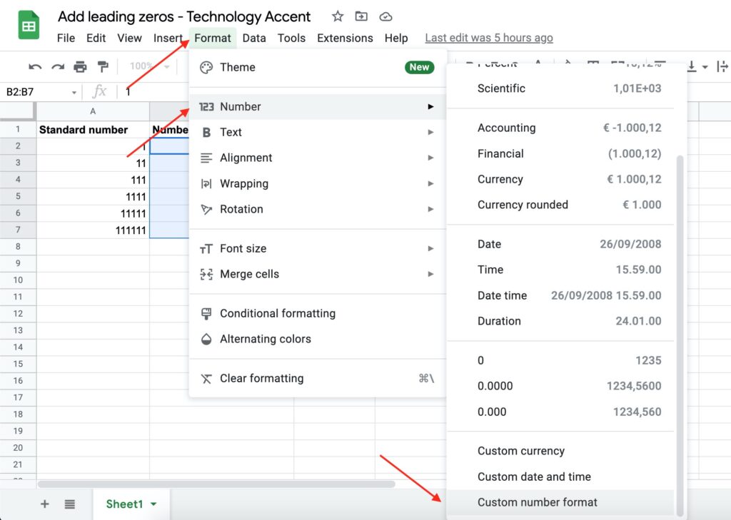
- Now you should enter the custom format code for your numbers. In my example, I will add leading zeros to get all 7 digits numbers, so I enter 0000000 in the format box. The total number of characters of the custom format code should be your desired length, composed of zeros, and a # as the last character.
- Once you entered the right format code, click on the Apply button to confirm.
- The result is a column of numbers with leading zeros added to get to 7 digits numbers.
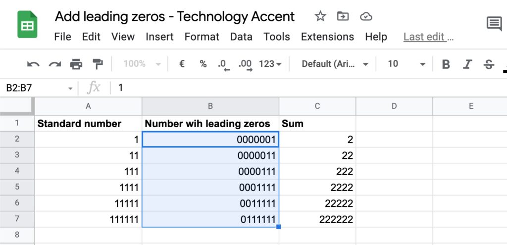
- Also, you can see that the sum column is still valid, as the numbers are still numeric values.
This is by far the best and simplest method to add leading zeros without losing the number format and the one you should use unless you have special needs.
This article is part of our productivity tips for Google Sheets series. You can find them all on our Tips and tricks for Google Sheets page.
Adding leading zeros with the QUERY function
While researching to write this article, I found this strange method. It’s a workaround you should probably avoid, as I can’t see a situation where this solution is better than the previous method.
But we are technology enthusiasts, so let’s see this strange method even just for completeness’ sake.
We are going to need to use the QUERY function. To take a value from a cell, and write it on another cell with the added zeros.
In my example, I will take the numbers in column A, and put the result of the query function in column B.
The formula I need to enter is:
= QUERY ( A2, "SELECT * FORMAT A '0000000'" )Then you can drag the formula on the other rows, or leverage the fact that the Query function works with arrays, so in my example, I can write:
= QUERY ( A2:A7, "SELECT * FORMAT A '0000000'" )And get all the rows populated directly.
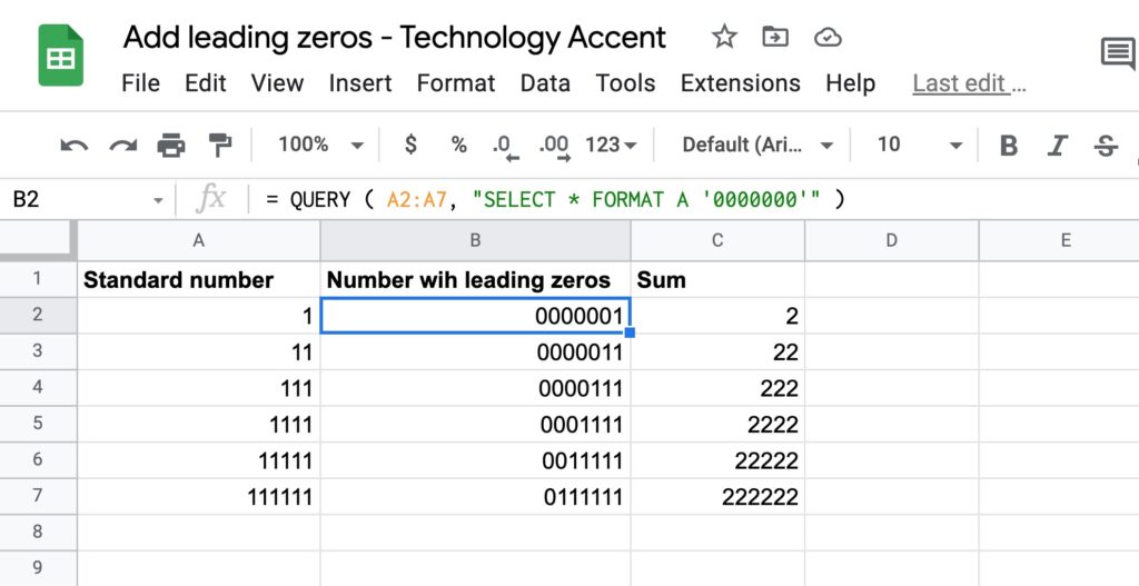
With this method, the number is preserved as a number, so the sum is working.
Adding leading zeros losing number format
When you don’t need to preserve the numerical properties of the cell, you can use a list of methods that add the leading zeros by transforming the cell format to text. This can be an easy solution where you don’t need your cell contents as numbers to use in formulas, like for employee ids, zip codes, and other similar types.
Let’s see some ways to add zeros in cells that will become text cells.
Using the apostrophe to convert to text
The easiest and quickest way to convert a number to text in Google Sheets (which also works in Microsoft Excel) is to put an apostrophe ‘ in front of the number.
Let’s see how to do it:
- Click on a blank cell.
- Put an apostrophe as the first character.
- Write your zero-prefixed string.
- When you’ll press the enter key, the number will be treated as text (and so will be aligned on the left by default) and the zeros will not be deleted.
A few additional notes:
The apostrophe will not show in the cell content, but you can see it on the formula bar if you select the cell.
As you can see, the sum column does not include the new cell content in the formula, as that cell is now text and not a number. This behavior is what we expect when using a method that transforms the content into text.
Using the plain text number format
We used the Format -> number menu in one of the previous methods while custom formatting the number.
There’s another option in that menu that comes in handy when you need extra zeros on your cell.
It’s the “plain text” option, that converts the format of cells to text as we did in the previous method, but without having to manually add the apostrophe to every single cell.
- Select the cell or range of cells you want to convert to text.
- Click on Format to open the Format menu.
- Go to Number to open the submenu.
- Select “Plain text”.
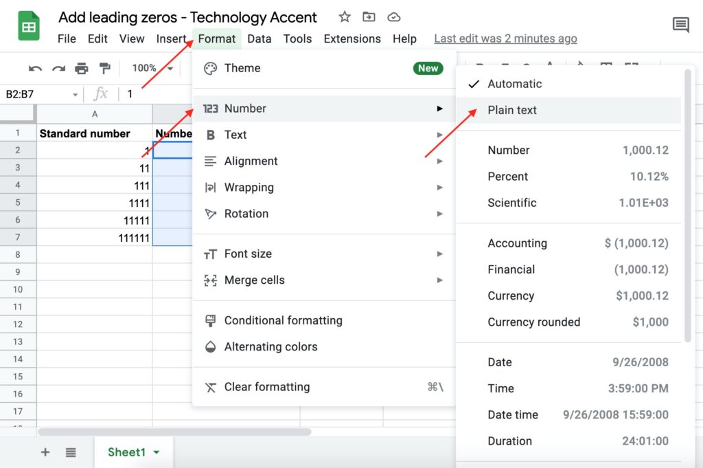
- The numbers will be converted to text, so you’ll see them left-aligned.
- This time there’s no number format code to enter, but you have to manually fill the zeros in every cell.
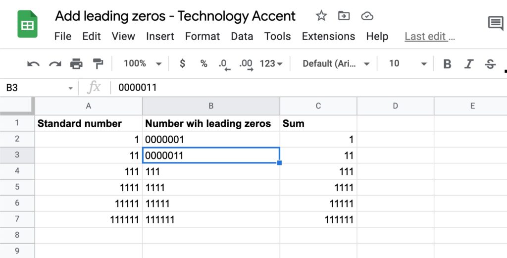
As we expected, the cell content has been transformed into simple text, so the sum column is ignoring it.
Using the TEXT function to automatically add the zeros
The methods above are good ways to solve the problem, but in both cases, you have to manually fill the zeros one by one.
The TEXT function is a solution worth considering if you want to avoid all the manual work.
However, everything comes at a cost: The TEXT function works really well if you have a cell reference to use to take the number from. It works with plain numbers, but using a cell reference is definitely quicker.
The syntax is simple:
=TEXT(number, format)So you have to use a number or a cell reference as the first argument, and a format for the second. The Format is the same as the one we previously used for the custom cell format method.
Let’s jump to our test spreadsheet and see a real example of this function in action:
- Select the cell you want to use.
- Write the TEXT formula. in my example I’ll write:
=TEXT(1, "0000000")- Press the enter key to confirm
- The result should be a string consisting of 7 digits like in the screenshot below.
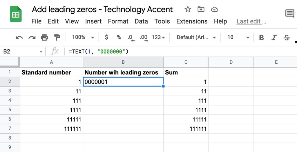
Let’s analyze a bit the syntax I used here:
=TEXT(1, "0000000")The first argument is the value I want to be padded with zeros. Here you can insert a cell reference if you want the number to be taken from another place (in my example I could use A2)
The second argument is the custom number format code to use. Include as many zeros as you need.
As in the other examples, this produces a text-formatted cell, so it’s not included in formulas.
This method is better if you use a cell reference instead of a plain number as the first argument, as you can easily drag the formula on an entire column, and editing the values is easier, you edit the source cell, and the target cell gets automatically updated.