One of the great advantages of using Google Sheets is the ability to work in a team/group editing the same shared file. However sometimes giving everyone the ability to edit the full document can be a problem, someone can accidentally edit the wrong cell and damage the document. Fortunately, Google gives us some simple and useful solutions!
How to lock a specific cell in Google Sheets?
If you want to protect your document, you can lock a single cell, so that other people can’t edit its content.
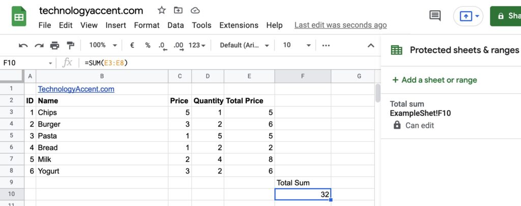
In our example, we have a simple document with some lines containing products, their price, a quantity, the total price, and finally the total sum of all the prices:
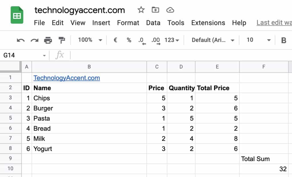
From this file, we want to lock the formula for the total sum, so we can share the document with someone and let him edit for example prices and quantities, but not the total sum.
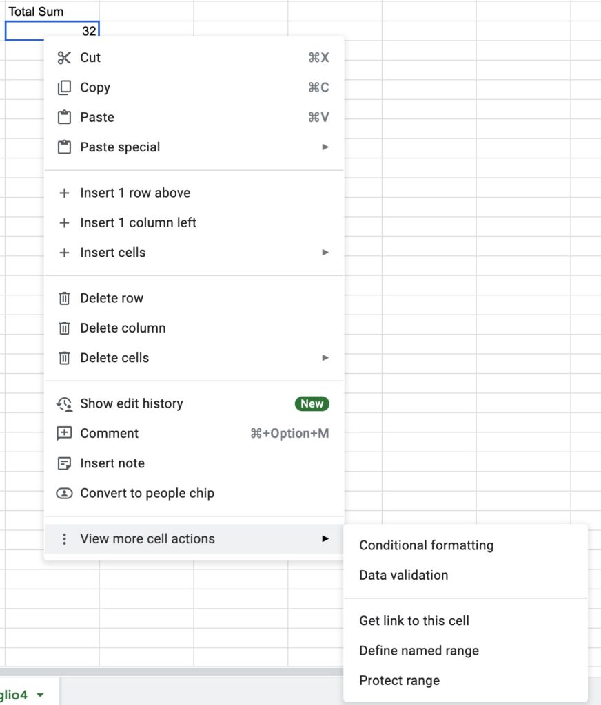
To lock a cell, you have to select it, then right-click on it, and select “View more cell actions” -> “Protect range”.
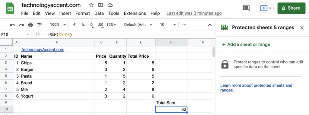
On the new side menu, you can choose “Add a sheet or range”.
In the next step, you can enter a description for the protection rule, so you can then be able to find it and remove the lock if you need.
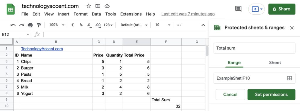
Check that the range field is the right one (in our example ExampleShet!F10) and click “Set permissions”.
In the next popup, you can choose if you want to give permission to someone to edit the range. For this example, we will completely restrict the access, so we select “Only you”. In the next examples, we will discuss the other options in detail. Once you’re done, click “Done”.
Now the locked cell will not be editable by others, and we can view the newly added rule in the “Protected sheets & ranges” window.
This article is part of our productivity tips for Google Sheets series. You can find them all on our Tips and tricks for Google Sheets page.
How to lock a range of cells in Google Sheets
Now that we know how to lock a single cell, let’s talk about cell ranges. The procedure is almost the same, so there will be fewer screenshots and more step-by-step textual instructions.
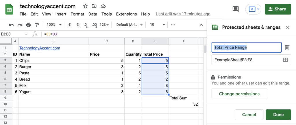
The first step is selecting the range of cells we want to protect. In our example we will lock the content of the “Total price” values, to avoid the formula being modified.
Then right-click on the range and select “View more cell actions” -> “Protect range”.
Check the Rule name and that the range is correct.
Click on “Set permissions”.
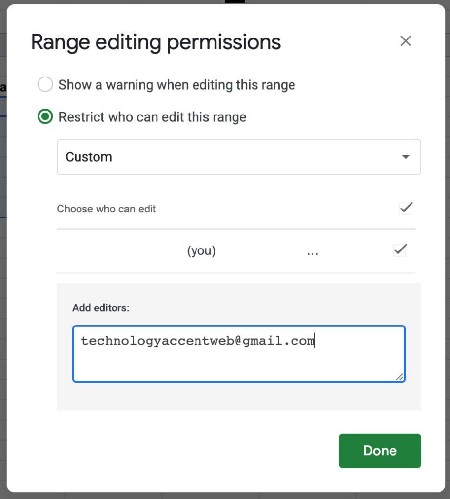
In our example, we will select “Custom” on the “Restrict who can edit this range” and add an additional editor.
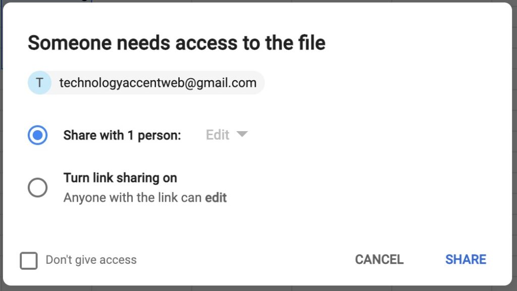
Once you click “Done”, if you added the email of a person you’re not yet sharing the file with, a new popup will appear to ask if you want to share the file with that account.
If you gave the edit permission you probably want to share the file too, so just click the “share” button to confirm.
Lock an entire sheet
If you need you can even lock an entire sheet. It can seem counterintuitive: why share if I don’t want anyone else to edit my data? But this is actually what most people do when they use Google Sheets. They share their spreadsheet with colleagues, but only allow them to make edits to certain parts of the sheet. And you could have a sheet with some data that you want to keep read-only, and another where you give your colleagues the ability to build formulas to extract data from the locked sheet. Or maybe the other way around, you prepare the sheet with all the calculations, lock it, and let the others input/edit the source data.
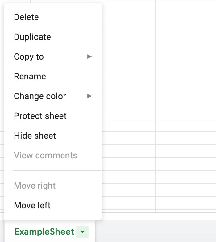
Locking an entire sheet is easy, you need to click on the down-pointing arrow near the sheet’s name, and select “Protect sheet”. A new “Protected sheets & ranges” will open with the “Sheet” option preselected. Just enter a description and click on “Set permissions”.
How to lock a column in Google Sheets?
If you want to lock an entire column you can do it easily. In our example, we may want to lock the “Price” column to avoid other users modifying the prices. We’ll start by locking the whole column.
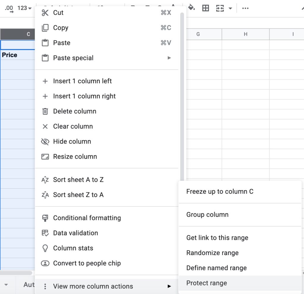
Select the column you want to lock (in our case the “price” column) and click on the down-arrow icon at the top right corner of the column or just right-click on the column header. Then select “View more column actions” -> “Protect range”.
A new window will appear asking for a description. Enter something like “Column price lock” and click on “Set Permissions”.
In the next step, you can choose the editing permissions just like you made for the range option.
How to lock a row in Google Sheets?
The procedure to lock a row is exactly the same as for columns. You just need to select the row instead of the column.
Select the row you want to lock and click on the row header (where you see the row number). Then select “View more row actions” -> “Protect range”.
A new window will appear asking for a description. Enter something like “Row 9 lock” and click on “Set Permissions”.
Soft locking cells with a simple warning
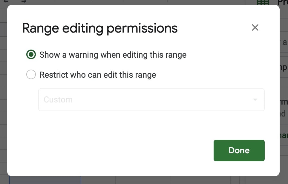
If you don’t want to completely lock the cell content, you can tell Google Sheets to just display a warning when someone tries to edit the cell ranges you protected.
To soft-lock individual cells or ranges, you just need to select the “Show a warning when editing this range” option in the “Range editing permissions” window. Once you click on done, everyone trying to edit the content will get a warning but could still modify the cell contents.
Opening the Protected sheets & ranges dialog to edit the protection settings
Ok, we just created a bunch of locked cells, range, columns, and everything, but now we want to edit permissions settings on those ranges. How do we do it? Let’s see step by step!
The “Protected sheets & ranges” window is accessible in the Data menu, just open it, and select “Protect sheets and ranges”.
The new window will show all the protected ranges. If you click on one of them, you’ll get to the settings, where you’ll find the Change permissions button, this will open the “Range editing permissions” and let you give or revoke permission to edit the range to another person.
How to unlock cells in google sheets?
As you can lock, you can unlock, let’s see how:
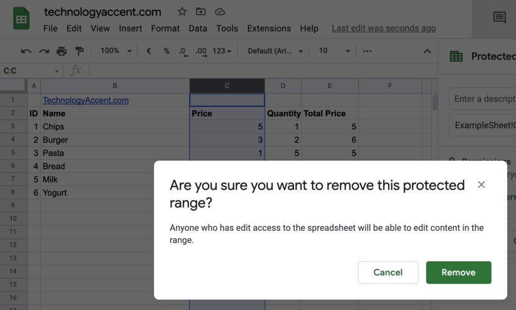
Open the “Protected sheets & ranges” from the “Data” -> “Protect sheets and ranges” menu item. Then click on the Range option you want to unlock and click on the trash bin icon near the Description textbox. A warning message will ask for a confirmation, click on remove and you’re done.
Conclusions
Locking and unlocking cells and ranges is a great feature that makes Google Sheets more flexible when ti comes to sharing work among team members. It also helps to protect your data from being modified by others without your approval.
There are many ways to protect cells and ranges in Google Sheets, so I hope this tutorial helped you understand how to use these.