I found myself in the need of merging two adjacent cells in google sheets without losing the data contained in them. I searched online and found everyone suggesting to download an addon. But then you discover the addon is not completely free, and I don’t want to give access to my data to an addon only to make a simple task. So I found an alternative method to merge two cells joining the content.
Avoid joining cells if you have formulas inside or referring to them
When we join two cells, we are forcing the spreadsheet’s rigid structure made of ordered and addressable rows and columns. This is not a great idea for cells containing data, as this can mess up selections, formulas, ordering, and filters. For these reasons, it’s better to use the merge function for “cosmetic” applications (titles, notes, etc.) and not in the data tables.
Creating a new temporary column
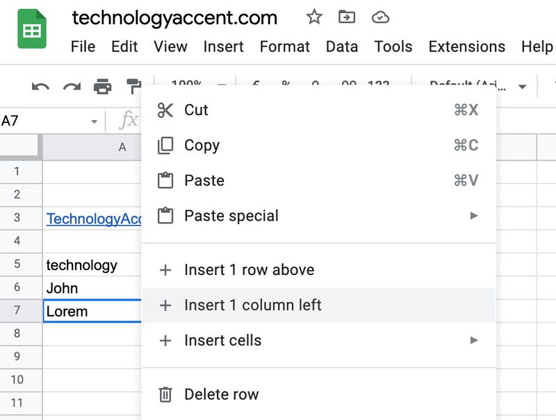
The first step is creating a new column we will use to temporarily merge the cell contents. This will be removed after the merge, so it’s not important where you place it. You could even put it on the first column of the sheet, but that would be more difficult to find later. I prefer to add it to the left or right of the cells I need to merge.
In our example, we will add it to the left as column A.
To do this we just need to right-click on the left cell and choose “Insert 1 column left”.
Merging the contents of the cells
Now we have to merge the two (or more) cells we want to merge.
Here it depends on what you want as a result. We have to write a function that merges the cell content as needed. You can concatenate the text of the individual cells, or if you have numeric values maybe you want the sum in the merged cell.
Whatever you want, you have to write a formula to get the result in the new column.
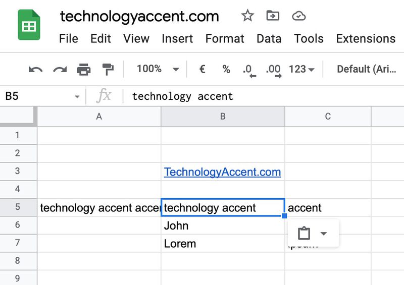
In our example, we will concatenate the values with a space character as a separator in the middle. A simple formula to merge values is the following one:
=CONCATENATE(B5;" ";C5)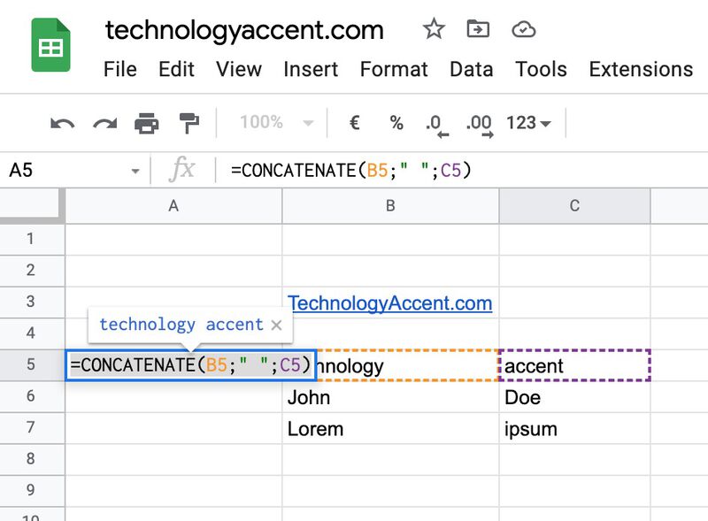
As you can see, the formula asks Google Sheets to concatenate the B5 cell’s content, our space separator, and the C5 content. You can use a different delimiter for the merge, such as a comma, or a comma and a space.
If instead you have numerical values and want to sum them, then you need to write a simple formula with the SUM function.
=SUM(B8:C8)
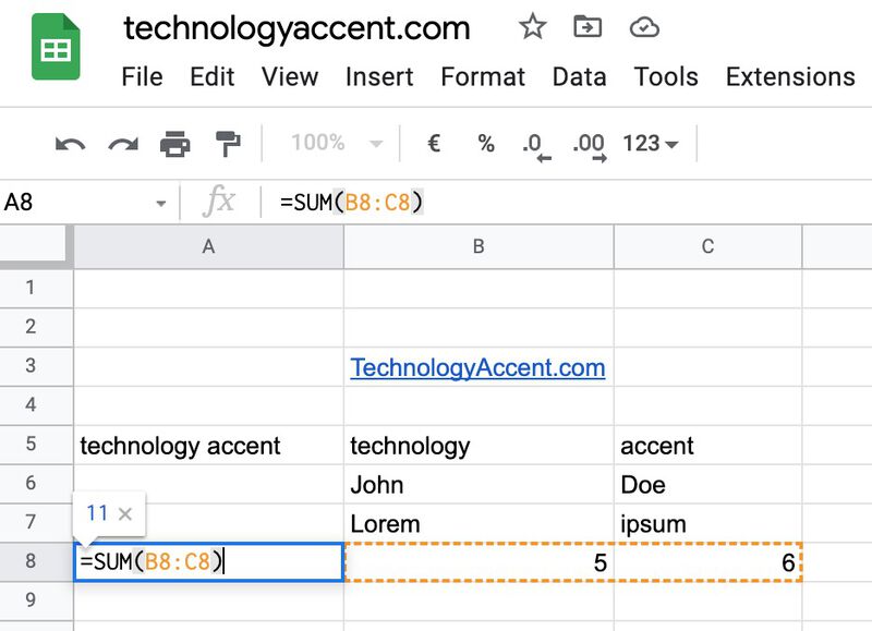
If you have to do the join on multiple rows, then you can just drag the formula to replicate it.
Copy the merged cell values to the top-left cell
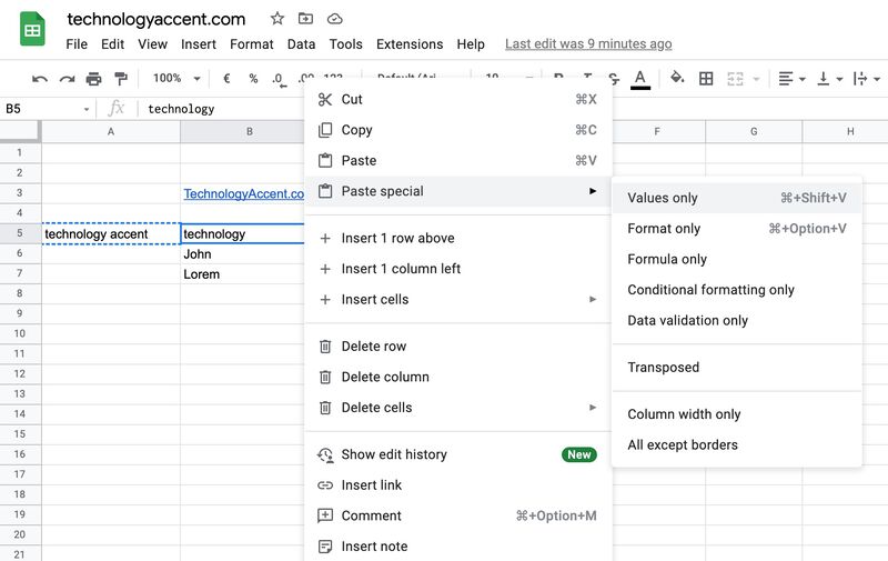
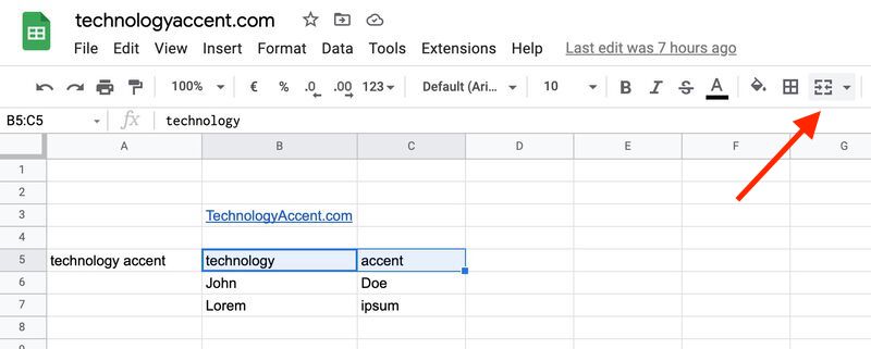
Now that we have all the data in the temporary cell, we have to copy it to the top-leftmost cell of the cells we want to merge. So in our example, we have to copy everything on the B column as we’re going to join the B5 and C5 cells.
Since the value we’re copying is a formula, and it’s involving the destination cell, we can’t just copy and paste from the helper column to the destination cell. The right way is to use the “Paste Special” -> “Values Only” option. This will paste the value instead of the formula. If you like keyboard shortcuts, you can use the Ctrl + Shift +v for Windows, and Command + Shift + v for Mac.
Once you pasted the content, the temporary cell will update the formula result and give a wrong value, but we don’t need it anymore.
Merge cells into a single cell
Now that we have all the data in the right place we can proceed to merge the cells.
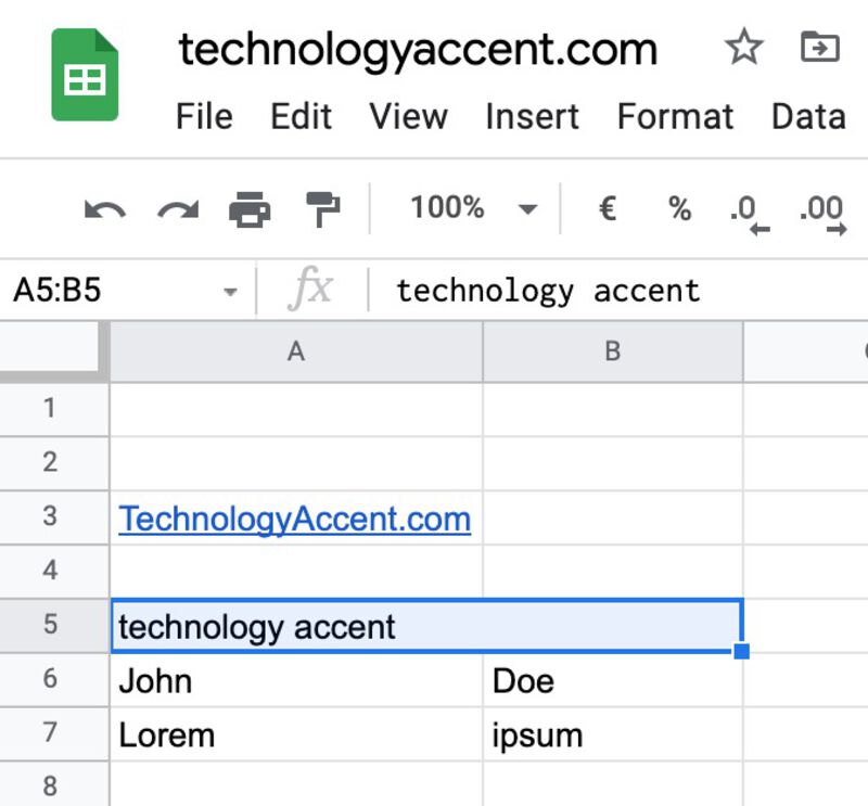
Google Sheets offers a simple way to merge the cells: You just need to select the range of cells you want to merge and then click on the “Merge Cells” button.
The default behavior of this operation is to keep only the content of the top-left cell, so if you have data in other cells that are being merged, you’ll get a warning from Google Sheets saying that you’re going to lose some data. Our data is in the right place, so we can ignore this message.

Once we confirm, the merge command will be executed, and the selection will become a single cell containing the right data.
Remove the temporary column
Now that everything is merged, we have to get rid of the temporary column.
You can select the entire column by clicking on it and then right-click and choose the “Delete column” option. Alternatively, you can select a single cell in that column, right-click on it, and use the “Delete column” from there.
This article is part of our productivity tips for Google Sheets series. You can find them all on our Tips and tricks for Google Sheets page.
How to merge two cells on the same column?
In our example, we merged in a row, but this method works in a column too, just create a temporary row instead of a column, and copy the merged values to the top of the array of cells you’re merging.
Conclusions
OK, it seems a long method, we all would like a merge feature from google sheets, but once you get familiar with it, it’s quicker than installing an add-on for just a simple feature.