OK, this is a pretty common task! Having a “name” and a “surname” column, and wanting both merged into a single “full name” column. And even if we’re making this specific example, you can use this guide to merge the content of two or more cells regardless of their content being names or something else. I think every google sheets user will need this sooner or later. I needed it so many times!
In this article we’ll see many ways to get this task done, probably you need only one, and probably there are many other ways, but the proposed ones should be enough for most of us!
Combine two cells in google sheets with the Ampersand Operator
This is probably one of the quickest, simplest to use, and easiest to remember ways to combine text from multiple cells into another one.
The ampersand operator (&) is used to combine two values, it simply combines what he finds on his left with what he finds on his right.
The first example will be an easy formula, just to combine the name and surname cells.
= A3 & B3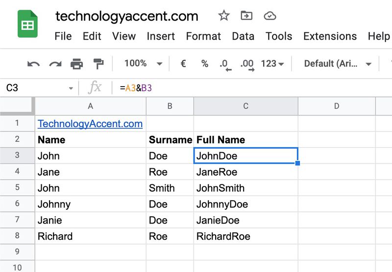
This is probably not the result we wanted, as the ampersand just merged the cells without using a separator between the values.
But what did we say earlier? the ampersand combines the left and right values joining them. We can use the & as many times as we want in a formula, and we’re not restricted to using it with cells, we can directly feed characters or strings to it. So let’s see how we can use it to combine first and last names properly!
=A3& " " &B3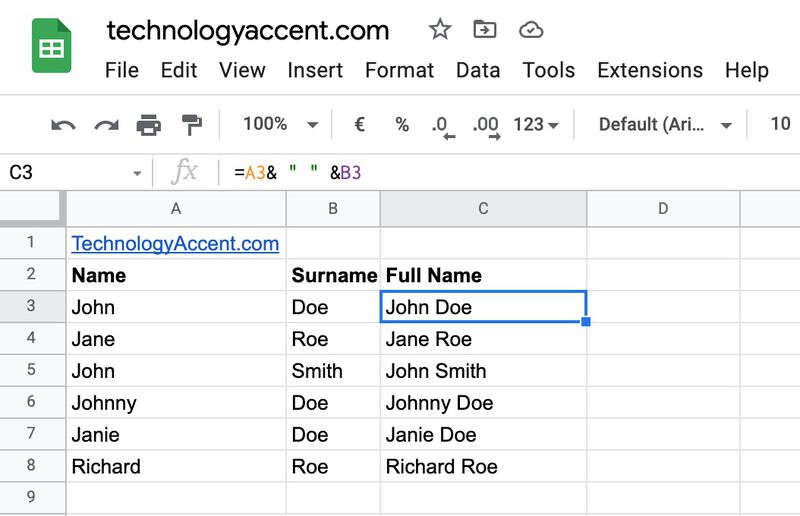
Ok, that’s better! We just used the Ampersand operator, but used it twice to concatenate with a space in the middle. We used a space character as a delimiter, but you can really use whatever delimiter you want, such as a comma, a dash, or a comma and a space. When you add the delimiter, just make sure to put it between double quotes, like “,” “-” or “, “.
This article is part of our productivity tips for Google Sheets series. You can find them all on our Tips and tricks for Google Sheets page.
Combine last and first name using the CONCATENATE function
The ampersand is probably the easiest way, but using CONCATENATE is probably cleaner.
We talked about the CONCATENATE function in our article about merging cells without losing data as a possible solution to another merging/combining problem.
Firstly let’s check the function’s documentation:
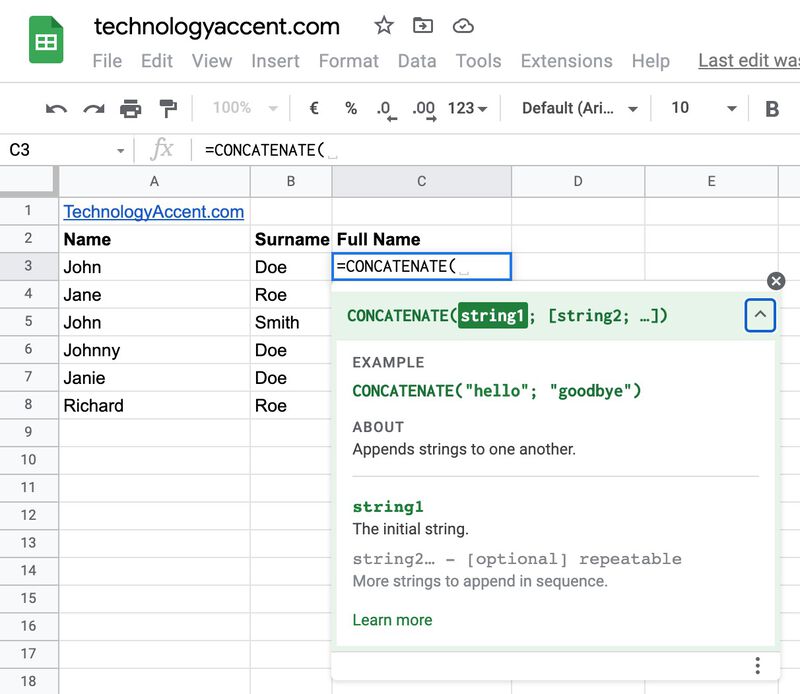
As we can see, the description says “Appends strings to one another”, and the function has at least one argument, but it can take many of them (actually 253, so probably more than you’ll ever need).
The example in the documentation is showing only two static strings, but we can give a reference to a cell as an argument. This is exactly what we need, let’s see how to use CONCATENATE in our example.
=CONCATENATE(A3; " " ;B3)This will concatenate the A3 cell containing the name, the space character (” “) and the B3 containing the surname.
This is the result:
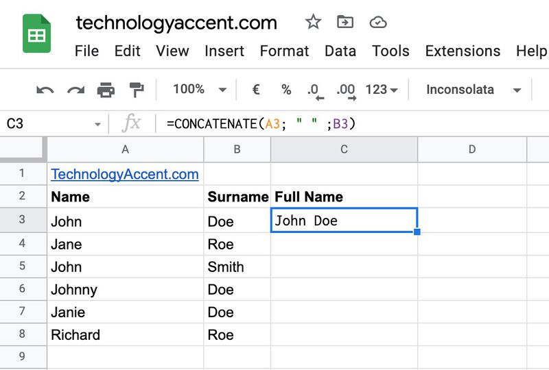
As in the Ampersand solution, we can use a different delimiter such as a comma or a dash. Always remember to double-quote the delimiter, or you’ll end up with an error.
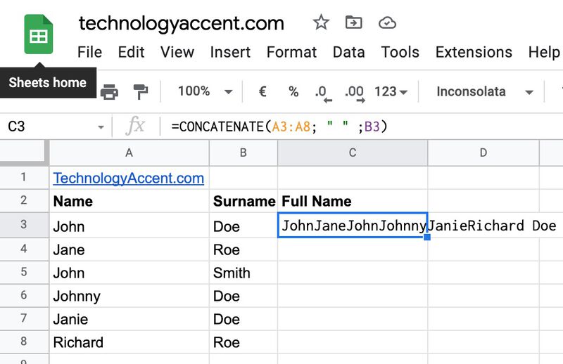
If you put ranges into the CONCATENATE function, it will automatically join all the values in the cells, and then use that value in the concatenate function. Be aware that the ranges will be joined without delimiters, using just the cell contents.
Use the TEXTJOIN function to merge two or more cells in google sheet
If you need to combine many cells into a single cell, then using TEXTJOIN could be a huge timesaver.
We’re talking about this as the third option and not the first only because it’s a bit more technical than the above-mentioned solutions.
Let’s go step by step, and see how TEXTJOIN works to merge cells before applying it to our example.
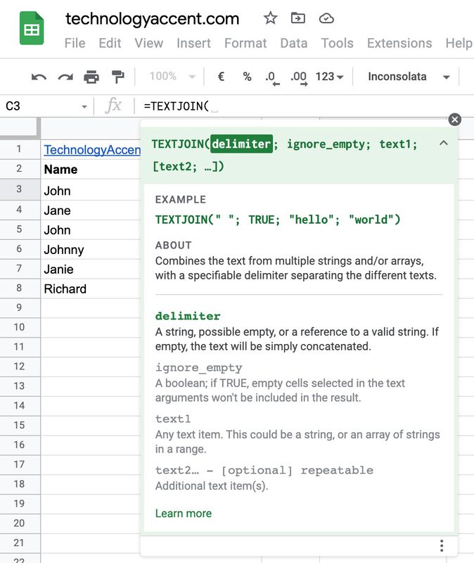
TEXTJOIN takes more parameters than the previous solutions, but it’s very flexible and powerful. Let’s analyze them one by one:
- delimiter: This is the delimiter we want to put between the cells. Here we can add our ” ” or “-” we used in the previous commands, simply there’s a field dedicated to the delimiter we want to use.
- ignore_empty: In this field, we need a boolean value (TRUE or FALSE) to tell TEXTJOIN if a blank cell should be ignored or used as an entry. If you set this to false, you’ll end up with a duplicated delimiter if a blank cell is found. Probably you’ll most likely always use TRUE to merge only non-blank cells.
- text1: The text we have to join. This can be a static text, a single cell, or a range.
- text2…: This indicates that we can add many texts that will be joined together.
Now that we know a little more about TEXTJOIN, let’s see how to apply it to our example to combine first and last names.
The functions we’ll use is:
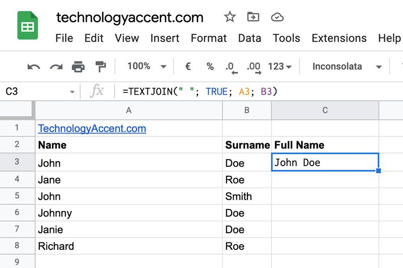
=TEXTJOIN(" "; TRUE; A3; B3)This tells google sheet to write in the destination cell the values from A3 and B3, using ” ” as a delimiter and ignoring the delimiter if one of A3 or B3 is a blank cell.
Using TEXTJOIN with ranges as arguments
TEXTJOIN can be used with ranges of adjacent cells instead of writing the cell references one by one. This interesting feature can be useful in our example, but it’s a huge timesaver with bigger ranges.
When we use a range in the arguments, the content of each cell is appended to the previous cells using the delimiter as a separator. Let’s see this in our example file, but to see better the advantages of this, we will combine all the names in the single column A, and separate them with a dash.
The formula to do this with the first method we explained would be:
=A3& "-" &A4& "-" &A5& "-" &A6& "-" &A7& "-" &A8It took me more than a minute, risked a lot of errors, and if I add a row, I have to update the formula with the new row cell reference. Not a pleasant experience.
We can rewrite the above with TEXTJOIN in less than 30 seconds, have the new row cell reference automatically updated, risk a lot more errors, and have a shorter, cleaner and scalable fomula:
=TEXTJOIN("-"; TRUE ; A3:A8)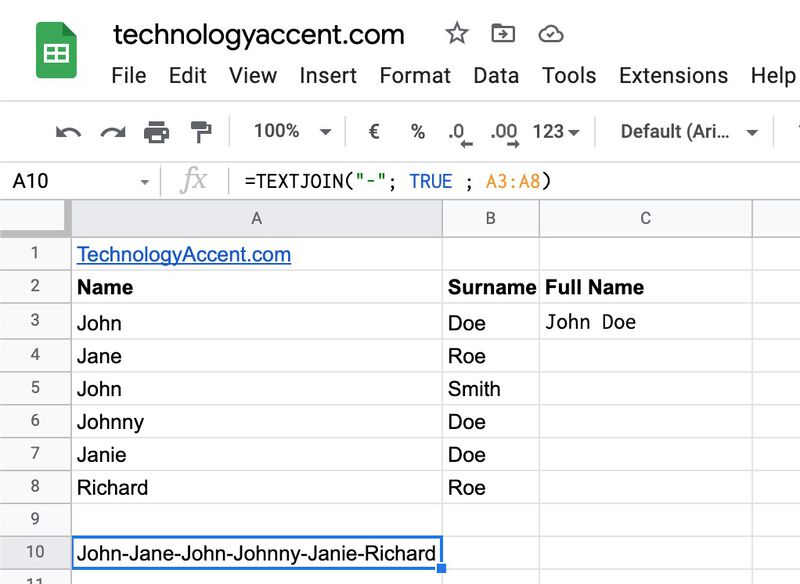
You can find the full documentation about TEXTJOIN on the google sheet support page
Let the autocomplete feature figure it out for you
Google sheet has a great feature called autocomplete or Smart Fill which uses an AI to try to understand your needs and do some repetitive work for you with a simple click.
In our example, if you move to column C and start to manually write the combined full names in the destination cell. While typing the second or third row, google sheet will pop up and ask you to step into this and complete the repetitive task for you. If you click to accept, the Smart Fill will do its work and fill the rest of the column for you.
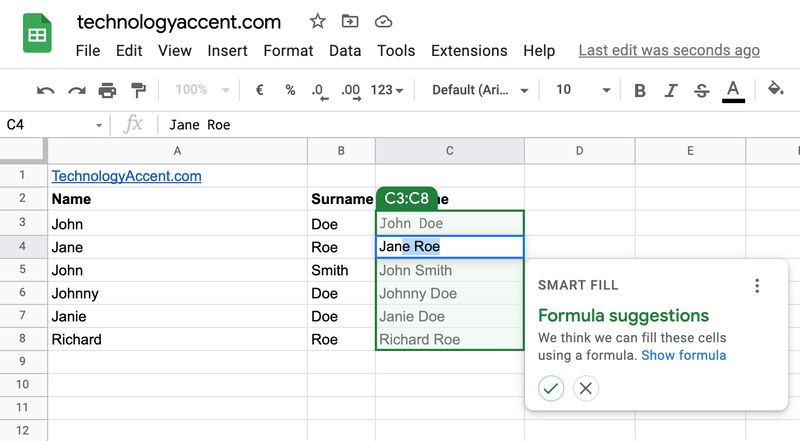
The Smart fill feature is pretty useful for long columns, as you don’t even have to manually drag the formula across cells.
Enabling the Smart FIll autocomplete feature on google sheets
The Smart Fill feature can be turned on and off, so if it’s not working for you it could be because it’s disabled.
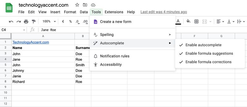
To enable Smart Fill on Google Sheets, open the Tools menu, choose Autocomplete, and enable the options you need (enabling all should be the way to go). From now, every time Google Sheets will have a suggestion, it will pop up and try to help you.
