Google Sheets strikethrough – Complete guide

Google Sheets is a great tool to save, organize and share data. It can be used for creating spreadsheets or documents that include tables, charts, formulas, etc. The most important thing about this great tool is the ability to easily add text formatting such as bold, italic, underline, strikethrough.

Sometimes you want to remove some text from a cell, but without losing it. This is when strikethrough comes in handy. You can cross out the text so it looks like it has been deleted. It’s like you would do it with pen and paper, but being a digital format option, you can revert it!

So keep reading to see how to strikethrough text in Google Sheets.

What is strikethrough?

Strikethrough is a formatting option used on almost all word processing programs, it’s a standard feature on almost every font, so you can find it almost everywhere you can format some text.

When you apply the strikethrough formatting to a text, the characters will be represented with a horizontal line crossing them. Here’s an example of a text with a strikethrough format applied:

This test has been crossed out with strikethrough

As you can see, the text is still readable, but the cross-out effect is evident.

Why use strikethrough instead of deleting text?

That’s the first question: why not delete text, but cross it out instead?

The reasons could be many. Maybe you want to remember the text, but exclude it when reading, or maybe you are correcting someone else’s work, and want to cross out it for removing, but you want to let the original author do it or at least know you don’t want that word/sentence.

Sometimes you may have a list of tasks or a list of things to buy, and you want to keep track of what you did/bought while preserving the original text. Think about a “monthly checklist”, you cross out during the month, and at the start of a new month, you just remove strikethrough and restart.

Add strikethrough with the keyboard shortcut

The quickest way to add strikethrough is by using a simple keyboard shortcut.

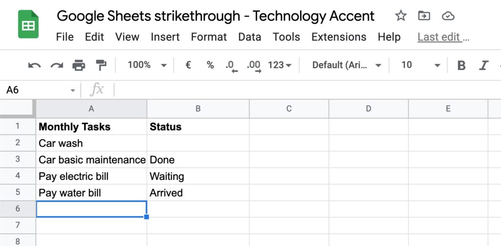
In our example, we have a simple list of monthly tasks, and we want to cross out the ones we completed.

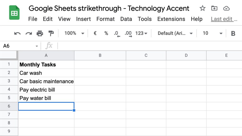
• The first step is selecting the cell with the text we want to strikethrough. I just completed my car’s basic monthly maintenance, so I’ll select cell A3;
• Then you have to use the shortcut <Alt> + <Shift> + 5 on Windows and Chrome OS.
• If you’re on a mac, there are various options and you have to find the one that works for your setup. The official keyboard shortcuts for Google Sheets page say you should use <Option>. + <Shift> + 5. However, this doesn’t work on my configuration, so I had to use one of <Command> + <Shift> + x, or <Command> + 5. 

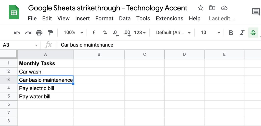
As you can see, the cell content is now crossed out, but if you see it in the formula bar, the text is shown without it, as it’s only a format option.

This article is part of our productivity tips for Google Sheets series. You can find them all on our Tips and tricks for Google Sheets page.

Adding Strikethrough from the Toolbar option

The next method is probably the most used, and easier to remember. Shortcuts are quick and easy, but not always so easy to remember and, for the features you use less frequently, it’s probably better to go with an easier-to-remember solution.

If you use Google Sheets regularly, you probably know and use the toolbar for other tasks, like changing text color, changing character size or font, and merging cells.

Let’s add another thing you can do with the toolbar!

This time I paid my electric bill, so I want to cross out that from my list of tasks.

• Click on the single cell or select a cell range if you need multiple cells.
• Click on the strikethrough format option from the toolbar, the icon with a crossed-out S.

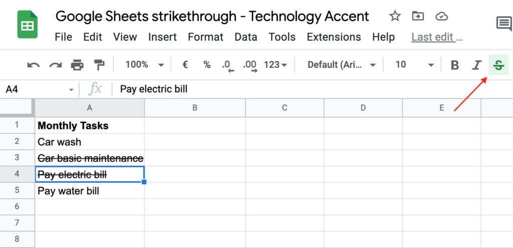
That’s it, now the electric bill is crossed out, we can stop worrying till next month! 

Add Strikethrough with the Format drop menu options

It’s probably a little longer to perform, but maybe a time will come when you’ll need to use it for some reason.

 If you like to use the menu bar for everything, you can use the Format menu!

Now, I just paid the water bill, and want to cross out that item on my spreadsheet so I don’t pay it twice.

I’m joking, I’ll not pay my bills twice, even without a checklist!

• Select the cell or range.
• Open the Format drop menu.
• Go into the Text submenu.
• Select the Strikethrough format option from the list.

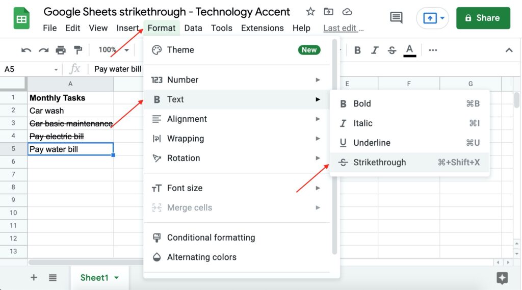
As you can see from the screenshot, on the right side of the strikethrough option, you’ll find the right shortcut to use, so the more you get to that strikethrough option in the menu, the more Google Sheets will remember you there’s a quicker solution you can use next time.

Add Strikethrough using Conditional Formatting

Ok, let’s get back to my example spreadsheet. I used it for some time, and I want to evolve to something more powerful. I want to add a “Status” column, so I can track every task’s status. For the bills for example I want to keep track when I am still waiting, when they arrive and are ready to be payed, and then when the task is done.

Keeping track of statuses and crossing out is too much for me, so I want to cross out the task when I write “Done” on the status cell.

Yes I know, all of this is overkill for 4 simple tasks, but it’s just to give you an idea with an example use case!

We’ll use Conditional formatting for this task.

This is our upgraded example spreadsheet:

• The first step is selecting the range you want to apply the conditional formatting to. I’ll select A2:A5.
• Next step is to open the Format drop menu.
• From the format menu click on the Conditional formatting option.

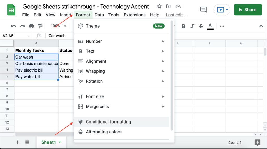
• The Conditional format rules panel will open with the Apply to range item pre-populated.
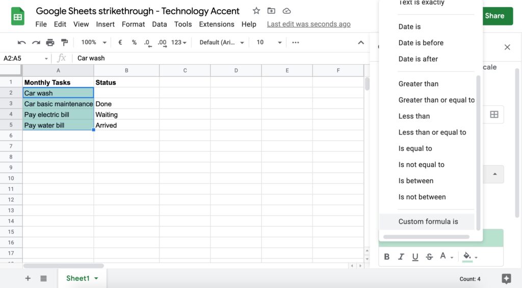
• From the “Format cells if…” drop-down menu select Custom Formula is (it should be the last option).

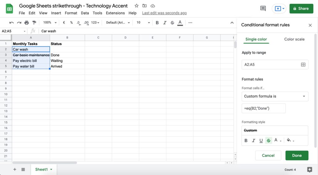
• In the Value or formula we have to enter the formula to decide if the Conditional formatting should be applied. In my case I’ll write =eq(B2;”Done”) so if in the B column I write the word Done, the formatting is applied to the corresponding cell on the left.
• In the Formatting style we can choose whichever formatting we want, in my case it’s pre-populated with a green background, so I’ll remove it by selecting None as the fill color, and click on the strikethrough icon to activate it. The Word “Custom” just below the Formatting style will update with the selected style.

• Once you’re satisfied with your formatting you can confirm by clicking on Done.
• Then you can also close the Conditional format rules panel.

 The conditional formatting is in real-time, so if you modify the content, the formatting updates automatically. In the screenshot, I have a task in Done status. If I remove it from cell B3, the cells with strikethrough will be reverted to standard formatting.

How to add Strikethrough on the android app

Sometimes you’re on the go, away from your computer, and want to edit your spreadsheet. You made your groceries checklist, and want to cross out the items you put in your cart.

But… where’s the strikethrough option on the Google Sheets Android app?

Let’s find out together!

• Open your Google Sheets document.
• Select your cell by tapping on it.
• Tap on the Text Format icon you can find on the top toolbar.

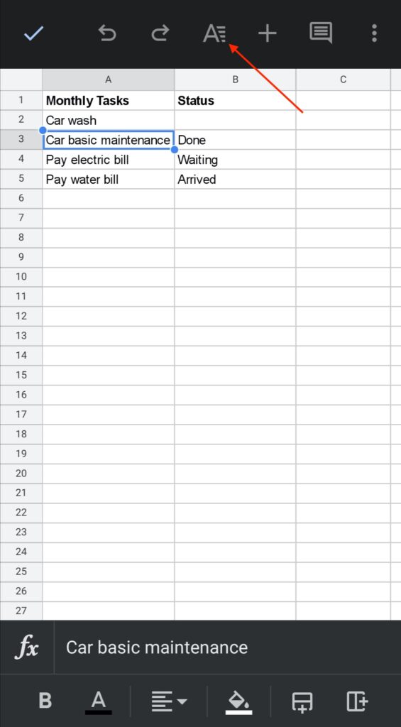
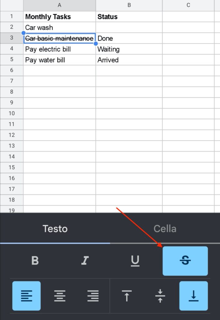
• A new bottom bar should appear with all the text formatting options.
• Tap on the strikethrough icon.

Now you can manage your task list/to-do list/whatever… even on mobile!

Remove Strikethrough Formatting in Google Sheets

OK… that’s interesting, all these methods to apply strikethrough… but what about removing it?

The great news is that the process is the same, so you can:

• Use the Keyboard shortcut methods: <Alt> + <Shift> + 5 on Windows, or <Option>. + <Shift> + 5 and <Command> + <Shift> + x on mac.
• Use the toolbar icon.
• Use the Format -> Text -> Strikethrough menu option.